Create a bit size curve from a caliper

Introduction

A caliper log records the borehole size. When a logging tool is pulled up the well, a caplier arm opens or closes as it encounters zones of washout, mudcake, or zones of stable hole condition. If there is abundant washout or mudcake, many logging tools (bulk density, neutron, etc.) do not collect valid petrophysical data. Often a petrophysicist will use some cutoff (2.5 inches of washout, maybe) to determine whether they can use the data over that interval in their analysis or if they should instead throw it out.

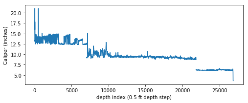
When a well is drilled, it is very common for there to be multiple “trips”, where a smaller bit size is used on each successive entry. As a result a caliper curve merged between logging runs will be stepped, as shown in this caliper vs. depth plot:

In order to assess whether our writeline data are valid or not, we need to compare the caliper to the bit size. The problem is that commonly bit size information is not available or is buried in rasterized records. When it is recorded in well metadata, it may not be precise (for any number of reasons, for example drilling depth and wireline depth being slightly different due to variable stretch on the drill pipe versus the wireline tool), or it wasn’t recorded properly by the sleep-deprived logging engineer, or it may be incomplete (“I see bit size for the shallow section, but what about the deeper part of the hole?”).

In this post, I document one method of estimating bit size directly from the caliper curve using a chagepoint detection algorithm and some pandas magic.

Set up

First we use lasio, a good library by Kent Inverarity for working with LAS files as python objects, to create a las object. lasio also has a method for creating a pandas DataFrame from the LAS file ~A data section.

import lasio
import pandas as pd

las = lasio.read('example_caliper.LAS')
df = las.df().reset_index()

Note that while traditionally LAS files are tied to depth, I will be working with the DataFrame index. The x-axes in the following plots can be thought of as log depth; only, divide by 2 to get the actual depth, since the depth step is 0.5 ft (one sample every half foot).

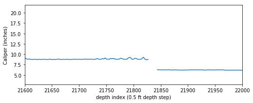
It is not uncommon to have null values in any logging curve, especially at casing points. In the figure above you can see the array has null values where the bit size shifts (namely at approximately indices 7000 and 21800). For this exercise to work we can’t have null values in our array, so we need to replace the nulls with numbers.

In this case we’ll select the CALI column from the dataframe, interpolate using the pad setting, and create a 1-D numpy array.

import matplotlib.pyplot as plt

plt.plot(df['CALI'])

signal = df['CALI'].interpolate('pad').values

plt.plot(signal)

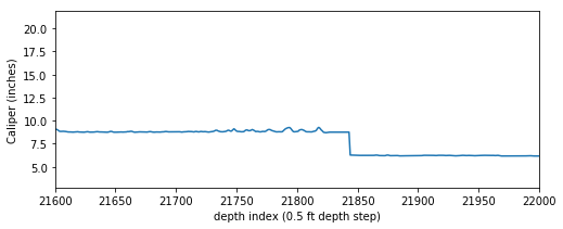
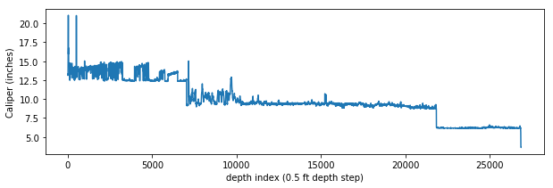
Here is the entire caliper curve from surface to the bottom of the well, with the interpolated values instead of nulls:

Changepoint detection

Glancing at the figure above, you can tell that an approximately 12-inch bit was used from surface to about 7000 depth index (since the sample rate on this log is 0.5 ft, that is about 3500 ft depth). There the bit was changed to ~9 inches then again changed to ~6 inches at ~22,000 depth index.

To the human eye, it’s pretty obvious where there are bit size changes. But if we needed to do this for hundreds or thousands of wells, that is an extremely tedious task to estimate bit sizes and the change points manually. This is where changepoint detection comes in (thanks to Jesse Pisel for the suggestion to try this technique).

There’s a nice library called ruptures that does changepoint detection. It has a familiar API to anyone with experience with scikit-learn which makes it quick to get up and running.

This is not meant to be a deep dive into the ruptures library. Instead, it’s just a proof-of-concept that this library can be effectively used to detect the major shifts in the caliper log that represent changes in drill bit size. In this case I’m using the BottomUp detection method and the l2 model, but there are several others built in to the library– you can read about the other detection methods and the other models that can be applied from the rupture documentation.

In this case I know the number of breakpoints and set the model to predict the changepoints at two places (i.e. n_bkps=2).

import ruptures as rpt

# instantiate model, fit it to our data, and predict the breakpoint locations
model = "l2"  # "l1", "rbf", "linear", "normal", "ar"
algo = rpt.BottomUp(model=model, jump=10).fit(signal)
my_bkps = algo.predict(n_bkps=2)

# show results
rpt.show.display(signal, my_bkps, my_bkps, figsize=(10, 3))

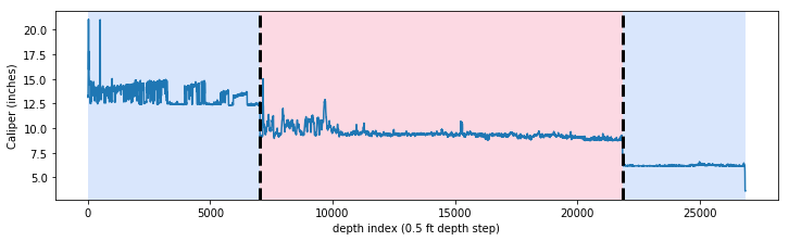
That worked pretty well! It took about 10 seconds to run with jump=10. ruptures has a built in method for creating a matplotlib plot with the breakpoints drawn and distinct regions of the curve shaded.

What if we don’t know the number of breakpoints? ruptures can deal with this as well. You can feed a penalty parameter to the predictor to tell the algorithm when to stop searching for more breakpoints. After a few trial and errors, I settled on a sigma of 20 for the automated breakpoint enumeration, which gave me the same number of breakpoints as above.

import numpy as np

sigma = 20 # acceptable standard deviation for this exercise
dim = signal.ndim
n = len(signal)
my_bkps = algo.predict(pen=np.log(n)*dim*sigma**2)

Create a bit size curve

We’ve found the break points thanks to ruptures. Next we want to create a bit size array to add to our LAS file. One of the outputs from the model prediction is an array with the breakpoints listed:

my_bkps

[7040, 21840, 26864]

We can create a list of bins for use in creating the bit size array from scratch:

indices = [0] + my_bkps
bins = list(zip(indices, indices[1:]))
bins

[(0, 7040), (7040, 21840), (21840, 26864)]

The amazing pandas library has a neat class called IntervalIndex. We’ll instantiate one of these using the bins we just came up with.

ii = pd.IntervalIndex.from_tuples(bins, closed='left')

Since we’ve been working in index space rather than depth space, we’ll use the cut() method on the DataFrame index to create a new column called BIN. By assigning the IntervalIndex object we just created to the bins kwarg, cut() will evaluate each row’s index and assign it to a bin based on the intervals defined in the IntervalIndex:

df['BIN'] = pd.cut(df.index, bins=ii)

Now every row of the dataframe belongs to a group which corresponds with the intervals we came up with using the ruptures library.

Remember, the caliper is the true borehole diameter as measured by the caliper arm on the logging tool and the bit size is the ideal borehole diameter. The idea is that if we compute a low percentile value of the caliper, we will be pretty close to the bit size:

df.groupby('BIN')['CALI'].describe(percentiles=[0.02])['2%']

BIN
[0, 7040)         12.348
[7040, 21840)      8.793
[21840, 26864)     6.141
Name: 2%, dtype: float64

So this describes the approximate bit sizes over the intervals: bit sizes used in this well appear to be about 12.3, 8.8 and 6.1 inches.

Let’s take those values and put them in a numpy array:

bits = df.groupby('BIN')['CALI'].describe(percentiles=[0.05, 0.02])['2%'].values

Drill bits typically come in standard sizes, and are usually relatively consistent across a region (though they may vary from basin to basin or continent to continent, onshore to offshore, etc.).

Having looked at dozens of well log headers in this basin, I have a pretty good idea of the bit sizes encountered. So here we’ll create a little dict with some common bit sizes.

bit_sizes = {
    6.125: 6.125,
    6.5: 6.5,
    7.875: 7.875,
    8.5: 8.5,
    8.75: 8.75,
    12.25: 12.25,
}

Now we look up which bit size each of the apparent bit sizes is closest to using that dictionary of standard bit sizes. To do so we pick the key where the magitude of the difference between the apparent bit size and the key in minimal. This is not very efficient but there aren’t many bit sizes nor many apparent bit sizes, so it is pretty fast despite the computational complexity.

estimated_bits = []
for i in bits:
    bit_ = bit_sizes[min(bit_sizes.keys(), key=lambda k: abs(k-i))]
    estimated_bits.append(bit_)

categories = dict(zip(df.BIN.unique(), estimated_bits))
categories

{Interval(0, 7040, closed='left'): 12.25,
 Interval(7040, 21840, closed='left'): 8.75,
 Interval(21840, 26864, closed='left'): 6.125}

There may be a better way to do dict lookup to go to a new column in pandas, but this apply() method, even though it’s not a vectorized operation, is fast enough for my purposes. The result is a column that records the bit size.

df['BITSIZE'] = df.apply(lambda x: categories.get(x.BIN), axis=1)

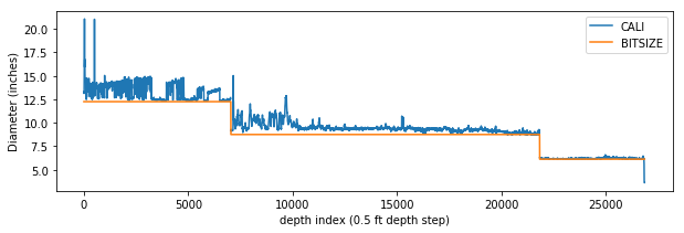
So, now we have a bit size curve. Here’s what it looks like when plotted alongside the caliper log.

plt.plot(df['CALI'])
plt.plot(df['BITSIZE'])

Update the LAS object and write to a LAS file

To finish, let’s create a new DataFrame with just the columns we want to send back into the python las object. We can do so by using the set_data_from_df() method.

df2 = df[['DEPT', 'CALI', 'BITSIZE']].set_index('DEPT', drop=True)
las.set_data_from_df(df2)

Write the las object to an LAS file and we’re done!

with open('bit_size_added.LAS', 'w') as f:
    las.write(f)